Developing a package to analyze data of the hospital morbidity survey

Installing the package

devtools::install_github("rOpenSpain/MorbiditySpainR",quiet = TRUE)
suppressPackageStartupMessages(library(MorbiditySpainR))
suppressPackageStartupMessages(library(lubridate))
suppressPackageStartupMessages(library(dplyr))
suppressPackageStartupMessages(library(ggplot2))
suppressPackageStartupMessages(library(geofacet))

Downloading data

I want to get a dataset light enough to do some descriptive analysis with my personal laptop so I dowload data from 2010 to 2014.

if(!file.exists("data.rds")){
  data <- GetMorbiData(y1 = 2010,y2 = 2014)
  saveRDS(data,"data.rds")
} else {
  data <- readRDS("data.rds")
}
dplyr::glimpse(data)

## Observations: 23,069,431
## Variables: 10
## $ prov_hosp     <int> 1, 1, 1, 1, 1, 1, 1, 1, 1, 1, 1, 1, 1, 1, 1, 1, ...
## $ sexo          <int> 1, 1, 1, 1, 2, 2, 1, 1, 1, 1, 2, 1, 1, 2, 2, 2, ...
## $ prov_res      <int> 1, 1, 1, 1, 1, 1, 1, 1, 1, 1, 1, 1, 1, 1, 1, 1, ...
## $ diag_in       <int> 1, 1, 1, 1, 1, 1, 1, 1, 1, 1, 1, 1, 1, 1, 1, 1, ...
## $ diag_ppal     <chr> "3019", "3770", "5532", "2851", "8518", "7865", ...
## $ motivo_alta   <int> 1, 1, 1, 1, 1, 1, 1, 1, 1, 1, 4, 1, 3, 1, 1, 3, ...
## $ estancia      <int> 3, 1, 2, 1, 1, 2, 1, 2, 2, 4, 5, 20, 1, 3, 6, 1,...
## $ cie           <dbl> 9, 9, 9, 9, 9, 9, 9, 9, 9, 9, 9, 9, 9, 9, 9, 9, ...
## $ fecha_ingreso <date> 2010-08-29, 2010-04-30, 2010-04-29, 2009-12-31,...
## $ edad          <int> 55, 90, 60, 45, 62, 55, 61, 66, 25, 46, 100, 46,...

Exploratory analysis

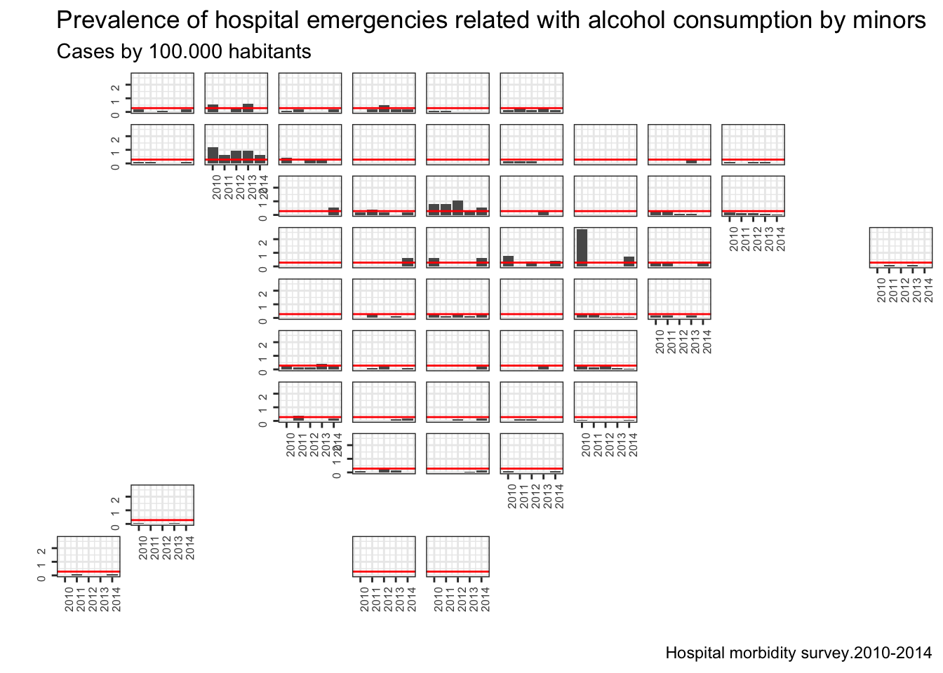
Regrettably we have an issue here in Spain with consumption of alcohol by minors, some times this consumption may end up in a hospital emergency, so let’s find out this in our data.

data <- readRDS("data.rds")
ll <- data %>% filter(year(fecha_ingreso)>=2010)

ll2 <- ll %>% FilterEmergency() %>% filter(edad<18) %>% FilterDiagnosis2(35)
ll2 <- ll2 %>% AddDiagnosis3() %>% ReduceData(provincia = TRUE,date = "year",diag = "diag3")
diag2.35 <- unique(ll2$diag3)
diag2.35 <- diag2.35[grepl("alcohol",tolower(diag2.35))]
ll2 <- ll2 %>% filter(diag3 %in% diag2.35)
ll2 <- ll2 %>% SetPrevalence()
ll2 <- ll2 %>% dplyr::group_by(prov,fecha) %>% dplyr::summarise(total=sum(total.prev))
ll2$code <- sprintf("%02d",ll2$prov)
ll2$year <- year(ll2$fecha)
prov.graf <- geofacet::spain_prov_grid1
ll2 <- full_join(ll2,prov.graf,by="code")

ll2.media <- mean(ll2$total,na.rm=TRUE)

g <- ggplot(data=ll2) + geom_bar(aes(x=year,y=total),stat="identity",position="dodge") + geom_hline(yintercept = ll2.media,color="red") + facet_geo(~ name, grid = "spain_prov_grid1") +labs(title="Prevalence of hospital emergencies related with alcohol consumption by minors",subtitle="Cases by 100.000 habitants",caption="Hospital morbidity survey.2010-2014") + xlab("") + ylab("") + theme_bw() + theme(axis.text=element_text(size=6, angle=90),strip.text = element_blank(),strip.background = element_blank())
plot(g)

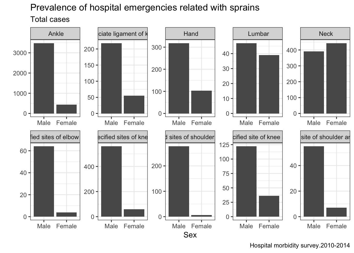
Another descriptive analysis we can do with dataset has the goal of knowing which are the most common sprain in people between 30 and 45 years, splitting resulst by sex.

data <- readRDS("data.rds")
lesiones <- data %>% FilterEmergency() %>% filter(edad>=30 & edad<=45) %>% FilterDiagnosis2(96) %>% AddDiagnosis3()
lesiones <- lesiones %>% ReduceData(provincia = TRUE,date = "day",diag = "diag3",sex=TRUE)

lesiones.y <- lesiones %>% group_by(diag=diag3,sex=sex) %>% summarise(total=sum(total))
esguinces <- lesiones.y %>% group_by(diag) %>% summarise(tt=sum(total)) %>% top_n(10,tt)
esguinces <- esguinces$diag
lesiones.y <- lesiones.y %>% filter(diag %in% esguinces)
lesiones.y$sex <- factor(x = lesiones.y$sex,labels = c("Male","Female"))

g2 <- ggplot(data=lesiones.y) + geom_bar(aes(x=sex,y=total),stat="identity",position="dodge") + facet_wrap(~diag,nrow = 2,ncol = 5,scales = "free") + labs(title="Prevalence of hospital emergencies related with sprains",subtitle="Total cases",caption="Hospital morbidity survey.2010-2014") + xlab("Sex") + ylab("") + theme_bw()
plot(g2)

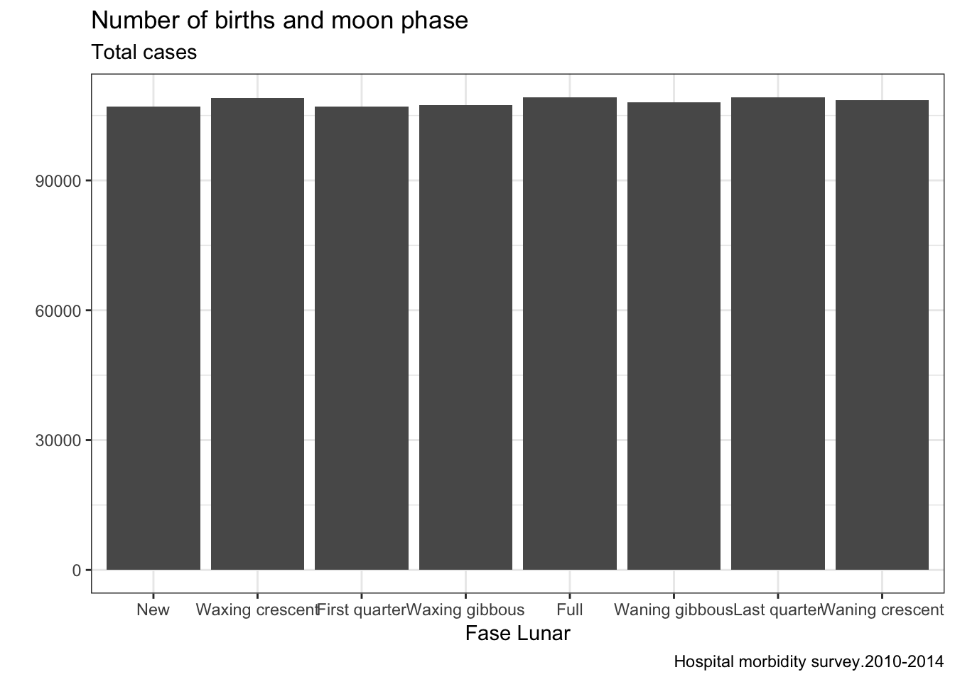
The next analysis imitates the famous Myth busters with data and answer the question of whether they are born more babies with full moon.

data <- readRDS("data.rds")
partos <- data %>% FilterEmergency() %>% FilterDiagnosis2(77) %>%  ReduceData(provincia = FALSE,date = "day",sex = FALSE)
library(lunar)
partos$phase <- lunar.phase(partos$fecha,name=8)
partos <- partos %>% group_by(phase) %>% summarise(total=sum(total))

g3 <- ggplot(partos) + geom_bar(aes(x=phase,y=total),stat="identity",position = "dodge") + labs(title="Number of births and moon phase",subtitle="Total cases",caption="Hospital morbidity survey.2010-2014") + xlab("Fase Lunar") + ylab("") + theme_bw()
plot(g3)

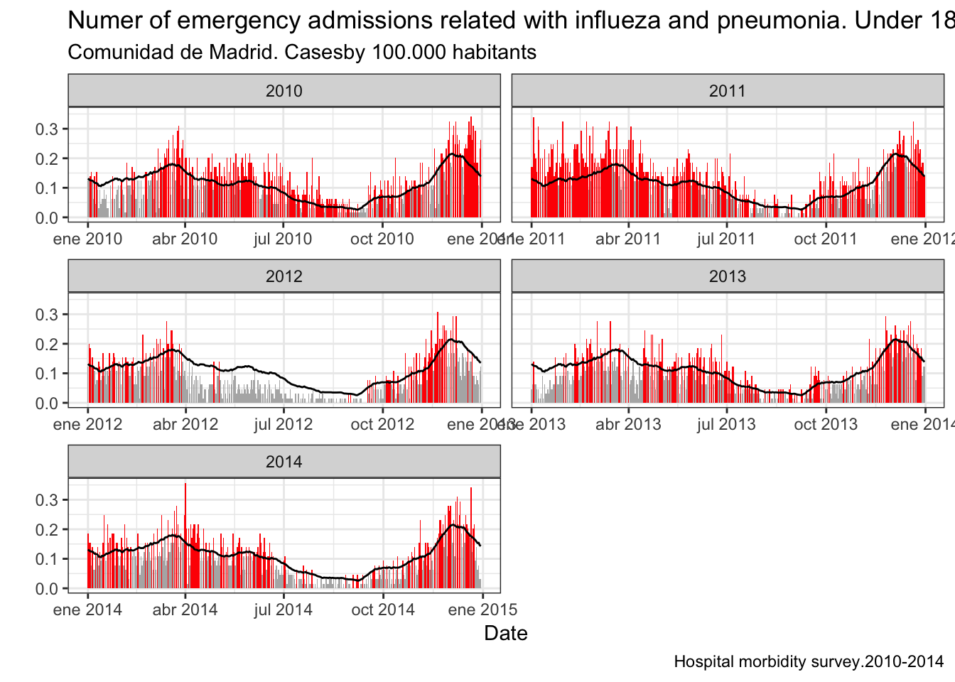
The last example builds a temporal series of hospital admissions of minors related with repiratorial diseases (flu and pneumonia) in Madrid. With this temporal serie we can construct a mean serie and compare them both to find epimediological episodes.

library(zoo)
data <- readRDS("data.rds")
ll.gripe <- data %>% FilterProvincia(28) %>% FilterEmergency() %>% dplyr::filter(edad<18) %>% FilterDiagnosis2(57) %>% ReduceData(provincia = TRUE,date="day",sex = FALSE) %>% SetPrevalence(pop = "total")
ll.gripe$yday <- yday(ll.gripe$fecha)
ll.gripe.clim <- ll.gripe %>% dplyr::group_by(yday) %>% dplyr::summarise(mean=mean(total.prev,na.rm=TRUE))

ll.gripe.rollmean <- bind_rows(ll.gripe.clim,ll.gripe.clim,ll.gripe.clim)
ll.gripe.rollmean <- rollmean(ll.gripe.rollmean$mean,15,fill=NA)[367:732]
ll.gripe.clim$mean <- ll.gripe.rollmean

# g4 <- ggplot(ll.gripe.clim) + geom_line(aes(x=yday,y=mean))
ll.gripe <- full_join(ll.gripe,ll.gripe.clim,by="yday")
ll.gripe$color <- ifelse(test = ll.gripe$total.prev>ll.gripe$mean,"si","no")
cols <- c("no" = "gray70", "si" = "red")
ll.gripe <- ll.gripe %>% dplyr::filter(year(fecha)>=2010)
g4 <- ggplot(ll.gripe) + geom_bar(aes(x=fecha,y=total.prev,fill=color),stat="identity",position = "dodge") + geom_line(aes(x=fecha,y=mean)) + facet_wrap(~year(fecha),ncol=2,scales = "free_x") + scale_fill_manual(values=cols,guide=FALSE) + labs(title="Numer of emergency admissions related with influeza and pneumonia. Under 18 years",subtitle="Comunidad de Madrid. Casesby 100.000 habitants",caption="Hospital morbidity survey.2010-2014") + xlab("Date") + ylab("") + theme_bw()
plot(g4)